Multi-Agent Coordination
Introduction
The research work I conducted in Multi-Robot Coordination (MRC) was the subject of my doctoral thesis. MRC may be defined as the planning, direction, and control of a team of multiple autonomous robots in a common environment to carry out a task, or multiple tasks, to achieve a common, global-level goal. Teams of autonomous robots can be made to efficiently and expeditiously perform tasks such as area-exploration, surveillance, mapping, foraging, etc., and MRC methodologies for these applications have been addressed in the literature. However, another application where autonomous robots can be beneficial is in the search aspect of Search and Rescue (SAR) operations. The advantages of using autonomous robots (for example, UAVs, as shown in Figure 1) in search operations can include their ability to: effectively move over rugged terrains, access highly confined areas, and provide consistent operation (compared to a human). As echoed by existing research efforts in this area, the increased automation of the search process can significantly improve the efficiency and success-rate of SAR operations.

Figure 1: Unmanned Aerial Vehicles (UAVs) can provide greater flexibility for maneuvering over difficult terrain.
The primary focus of much of the research on the automation of SAR has been on Urban Search and Rescue (USAR). USAR refers to search activities amidst collapsed structures after disasters and is concerned with locating stationary survivors within a bounded search area. Research interest has been shown in the design of various, often unconventional, mobile robots to deal with the particular challenges presented by USAR scenarios; Figure 2 shows one such example. Effort has also been placed on addressing human-robot interaction issues that arise in the tele-operation of robots in USAR applications. My research, however, dealt with multi-robot coordination for automating the search process in Wilderness Search and Rescue (WiSAR), a subject that has received relatively less attention in the literature. In WiSAR, the lost person (target) is mobile, moving in a non-deterministic fashion that can, nevertheless, be predicted in some way. Since the boundaries of the search area must grow as the target moves, the search environment in WiSAR is also potentially boundless. Moreover, one must also account for the effect of the target’s particular physiology, given the varying terrain that he/she potentially traverses, as well as the target’s lost-person psychological behavior, to accurately predict the target’s motion. This prediction must, then, be used to determine how to move the robots in order to maximize the chances of finding the target in the shortest amount of time. Through continued efforts in the development of such a method, one can envision a future where human WiSAR personnel are augmented with teams of autonomous robots to help with the search operations.

Figure 2: An innovative “Snake Robot” design integrated with a wheeled mobile-robot platform, being tested within the rubble of a mock collapsed structure at the NASA Ames Research Center (image used by permission from Dr. H. Choset, from the Biorobotics Laboratory at the Carnegie Mellon Institute).
Thus, in my thesis, I set out to develop a methodology to coordinate a team of robots to autonomously perform a search for a missing person in WiSAR scenarios. A key criterion throughout this research was to develop an approach that is feasible as an on-line method, since the intent was to have the method perform autonomously without the need for human intervention (except at the start of the search when the initial search-scenario data must be gathered and input into the central database). Hence, throughout the development of this methodology there have been instances where compromises have been made to the complexity of methods or to the attainment of global optimal solutions in favor of practicality and on-line feasibility.
In this methodology, a typical WiSAR scenario is assumed to proceed as follows: at a certain point in time, a notification arrives of a missing person. His/her last known position (LKP) is given, along with the time at which he/she was at this position. Basic topographic information of the region, as well as elementary knowledge of the personal characteristics of the target, such as age, clothing, provisions, purpose of visit, health, experience and familiarity with the area, are gathered before the search initiates. The available search robots are, then, transported to the LKP and arrive there at some later time. The total time passed since the estimate of when the target was at the LKP up to the time at which the robots arrive, represents the time for which the target has been moving from the LKP (i.e., the target’s “head-start”). The optimal initial deployment of the robots is determined a priori, and each robot may either be deployed directly at its optimal position, or all the robots may be released at a certain location and allowed to travel to their assigned deployment positions. Upon reaching their deployment positions, the robots are each assigned an optimal search path based on an analysis of all available information about the target and the search environment. The available information is updated throughout the search based on what the robots find, which, in turn, is used to regularly re-optimize and update the assigned search paths.
The problem, then, is certainly quite complex, and we address it by breaking it down into three main tasks:
1) Lost-Person Motion-Behavior Prediction;
2) Optimal Robot Deployment / Re-deployment;
3) Robot-Path Planning.
If approaches can be developed to autonomously perform each of these tasks, they can be integrated into an overall methodology that solves the MRC problem for WiSAR. In what follows, a brief description of the work that was done for each of these three main tasks is given.
Lost-Person Motion-Behavior Prediction
Foremost in conducting a meaningful search for a mobile (and non-trackable) target is to obtain some form of prediction of the target’s location. Moreover, since the target is moving, one must have a method for updating this prediction over time and space, based on some knowledge of how the target is likely to move. The objective of this first main task of the proposed MRC methodology, therefore, is to generate a probabilistic representation for the location of the target at any given time within a continually expanding search area. Although this may sound like a daunting task, it is not as hopeless as it may, at first, seem.
Certainly, it is unlikely that one can obtain a highly accurate prediction of the location of the particular lost-person being sought if the person is neither continuously nor intermittently observed. However, it is possible to use recorded search-data pertaining to similar lost-persons that were dealt with in the past to paint a reasonable picture of how the current target is likely to behave. Search and rescue organizations often keep records of key quantitative data gathered from past lost-person search incidents. This historical data is analyzed and organized according to different categories of the general type of lost person that was dealt with. Examples of such categories include: 1 to 6 year old children, hikers, hunters, skiers, fishermen, and despondent persons.
In reality it is quite difficult, if not impossible, to derive a 2-D, bivariate probability distribution for the location of a particular lost-person over a search area; how can one predict the trajectory that a lost-person would follow over time, or the probability that this person would move to any particular position within the search area? Existing probabilistic search methods will assume that such a 2-D probability distribution is available at the outset of a search. However, we do not make such an assumption. Instead, we use the abovementioned data that is readily available to predict the likely motion-behavior of the target being sought. From this we are able to derive a 1-D probability distribution for the location of the target along any single line of target-travel. This probability distribution is referred to as a target-location probability density function, or target-location PDF, for short. This, then, allows us to say something about where the target is likely to be at any given time within a 2-D search area as well. In particular, by making the conservative assumption that the target can move outward from the LKP in any direction according to the predicted motion-behavior, we can delineate multiple boundaries (closed, 2-D curves), each corresponding to a different probability of target-presence within the search area. Due to the use of conservative assumptions, these boundaries serve as upper bounds on the location of the target, thereby ensuring that we are at least able to enclose the target. As well, a means to propagate these boundaries over time and space to account for target motion has also been developed in our work.
These boundaries have been termed “iso-probability curves,” and they also serve as a novel representation mechanism for the available probabilistic target-location information. A simple example is shown at the top of Figure 3, where each curve represents the boundary of a different probability region. In this simple case, all curves are perfectly circular. The innermost curve bounds the region having a 10% chance of containing the target; the next larger curve bounds the region having a 30% chance of target-presence, and so on. The spacing between curves depends on the nature of the 1-D target-location PDF that is used to construct the curves. The curves in Figure 3 are based on a truncated Normal distribution (i.e., a symmetric and unimodal probability distribution), as shown by cross-section A-A at the bottom of the figure. Thus, although the curves are concentric, they are not equally spaced, even though the probability percentage increments between adjacent curves are all the same, namely, 20%. Hence, the curves may be looked at as the boundaries of the 2-D projections of different target-location probability regions onto the search area. Any number of curves corresponding to any combination of target-presence probability boundaries that are desired can be defined and portrayed in this way.

Figure 3: A simple example of iso-probability curves showing the boundaries of the 10%, 30%, 50%, 70%, and 90% target-location probability regions (top), and the 1-D target-location PDF on which these curves are based (bottom).
So, what can be done with these curves? Well, for one, they can allow us to incorporate the impact of a number of key influences on the target’s motion into the prediction and portrayal of the target’s probable whereabouts. In this work, three important influences in particular have been considered: terrain difficulty, target physiology, and target psychology. For example, Figure 4 shows the impact of incorporating terrain influence on a set of 10 iso-probability curves that are based on a Normal distribution for the target-location PDF. A set of key, defining points on the curves, called control-points, are shifted outward or inward relative to the LKP based on whether the terrain in each point’s vicinity tends to speed up the target’s motion (e.g., due to a decline in instantaneous terrain slope) or slow down the target’s motion (e.g., due to an incline). Computation of the amount of impact of the terrain topology on target motion would depend on knowledge of the target’s physiology – physical dimensions, general health, typical walking gait pattern (given their age), etc.
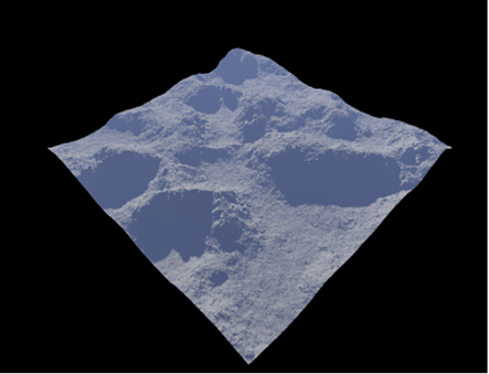
The terrain influence incorporated into the curves in Figure 4 was based on a computer-generated virtual terrain. These curves are one example among many others that have been used in various simulations conducted in Matlab®, where a selected set of iso-probability curves have been established and subsequently propagated over time and space. The TerragenTM Classic scenery-generation software was used to generate the different, realistic terrain topologies for these simulations. Figure 5 shows an example of a 3000 m × 3000 m mountainous region that was generated for use in some of the simulations.

Figure 4: Iso-probability curves modified to reflect the influence of terrain topology on target location.
(a)

(b)
Figure 5: A 3000 m × 3000 m area of mountainous terrain topology generated by Terragen™ Classic for use in simulations: (a) iso-metric view; (b) closer, horizon view.
Even aspects of target psychology can be incorporated into the target-location prediction using iso-probability curves. For example if the target is a lost tourist and somewhat familiar with the area, they may be aware of the existence and general directional bearing of a popular destination (such as a well-known village or chalet) where help and/or refuge can be obtained. This direction of travel, thus, becomes more likely compared to others, and is assigned a relatively higher probability, which can be used to “distort” the curves to reflect the impact of this high-probability direction. Figure 6 shows an example set of iso-probability curves for the case where the 0° direction of target-travel is the most probable.
In addition to incorporating the effect of these three influences on target motion, techniques have also been developed to alter the iso-probability curves whenever clues left behind by the target are encountered. This allows new information obtained from the search to be used to revise the target-location prediction and to modify the search strategy accordingly.
A third major utility of the iso-probability curve concept is that it can be used to help distribute the search effort. The particular curves selected for use can help to determine where, within the search area, the search effort should be placed, while the density of curves can guide the intensity of search effort applied to these areas. This is elucidated by the way in which the other two main tasks in the overall MRC approach are addressed.

Figure 6: Iso-probability curves modified to incorporate the influence of a probable direction of target-travel (high-probability direction indicated by dashed red arrow).
Optimal Robot Deployment / Re-Deployment
Optimal robot deployment refers to the process of determining how to distribute the robots within the search area of interest in order to maximize the chances of finding the target in the smallest amount of time. We distinguish the deployment process from the search process, treating deployment as a means of appropriately positioning the robots first, before applying a path-planning method to conduct the search.
More than just attaining a particular formation pattern, or maximizing the area covered under the robots’ sensors, the deployment problem in the context of an autonomous multi-robot search for WiSAR requires distributing the robots based on the available probabilistic target-location information. However, this information changes continuously due to the dynamic nature of the search, which is attributed to changes over time in the three key influences mentioned earlier, as well as to the incorporation of new information obtained from clues found throughout the search. Hence, to address this dynamic nature, one requires not only an optimal initial deployment at the start of the search, but also successive re-optimization and re-deployment during the search, in order to ensure that the robots remain optimally distributed within the search area as the prediction of the target’s location gets updated. As such, a specialized deployment method, different from what is typically considered to be deployment in the multi-robot coordination literature, had to be developed. The following briefly discusses the approach that we use to tackle this problem.
Since the concept of iso-probability curves was devised to represent the probabilistic target-location information, we link the deployment and re-deployment methods to this construct. In particular, each robot is assigned to an iso-probability curve and must attain a particular position on that curve to be considered deployed. Thus, a (re-)deployment solution entails specifying the number and position of iso-probability curves to use, and determining how to allocate the robots among these curves. In a more general sense, the specification of the iso-probability curves represents the selection of the regions within the search area where search effort is to be (re-)allocated, and the allocation of robots to these curves represents the (re-)assignment of search resources to those selected regions. However, in the case of re-deployment, upon obtaining a solution, there is still the question of how much benefit is to be had by implementing it. If this benefit is relatively insignificant, then a re-deployment solution would not be worth implementing, given the temporary, transient phase of disruption it would inevitably cause to the search that is in progress due to the sudden re-assignment of robots to a new set of curves to guide the search. As a result, the re-deployment problem that we deal with requires the consideration of two main issues:
1) Determination of the optimal search effort re-allocation;
2) Determination of the benefit of a re-deployment.
Initial deployment is simply a special case of re-deployment, in which the second issue of determining a benefit is not applicable, since the optimal solution obtained must be implemented in order to begin the search.
The problem of determining the optimal search effort re-allocation (i.e., optimal re-deployment) is modeled as a single-variable optimization problem, where the decision variable is the number of iso-probability curves to use. The positions of these curves, however, are selected using a pre-determined curve-placement strategy designed to preserve the logic and intent behind the optimal allocation of search resources. This approach simplifies method-execution and helps to ensure that it can be performed in an on-line manner. The objective function in this optimization is a quantitative measure of search effectiveness entailed by a given re-deployment solution, and is formulated based on a combination of three metrics relevant to the re-deployment problem in WiSAR: a measure proportional to the total time taken to find the target (search-time); a measure proportional to the probability of finding the target (success-rate); and a measure representative of the time required for the robots to reach their respective, assigned curves (return-time).
The presence of the third metric mentioned here may not seem as intuitive as the other two, but is necessary due to the way in which we address the WiSAR problem. The iso-probability curves are used to distribute the robots within the search area and to guide the robot search motions. Therefore, the re-assignment of robots to curves requires that the robots travel to, and assume a particular position on, their assigned curves, before continuing with their search motions as dictated by the planned search-paths. However, in general, at any intermediate point in time during the search, the robots will be distributed within the search area as they move about looking for the target using their assigned paths. As a result, when conducting a re-deployment optimization in order to find the new optimal set of iso-probability curves, some measure of the time that would be required by the robots to first travel to their newly-assigned curves before they can resume their search motions must be taken into account. To serve this need, the return-time metric was introduced.
Each iteration of the main (re-)deployment optimization evaluates a particular set of iso-probability curves and requires the computation of all three metrics. The computation of the return-time metric inevitably requires the determination of the optimal allocation of search resources (i.e., assignment of robots) to the set of curves being evaluated during that iteration. This entails specifying the number of robots that should be placed on each curve, as well as which robots, in particular, should be assigned to which positions on which curves in order to achieve this required number of robots per curve. This optimal assignment is determined so as to minimize the time that would be required by the robots to reach their curves and, in turn, is used to compute the return-time metric for that particular set of curves.
We, thus, propose a means by which each of these three key metrics, namely, search-time, success-rate, and return-time, may be formulated and normalized. Each metric is weighted according to user-preference and combined into a single objective function to drive the main re-deployment optimization. The final output is an optimal set of new iso-probability curves to use in the subsequent search, as well as the re-assignment of the robots to these new curves. Figure 7 shows a simple example of an optimal search effort re-allocation solution during a re-deployment. Here, 5 robots (blue dots) are optimally re-assigned to 3 curves (the 10%, 50%, and 90% iso-probability curves, respectively). The robot-requirements for the 10%, 50%, and 90% curves in this particular example are: 1 robot, 2 robots, and 2 robots, respectively. The magenta lines indicate the optimal re-assignments of robots to curves, and the magenta ‘×’s indicate the corresponding optimal re-deployment positions. It should be noted that, realistically, the robots would not generally follow straight-line paths to their curves as implied by Figure 7. Search-path planning is the subject matter of the third main task in the overall methodology. Still, the methodology limits itself to planning the general paths for each robot that simply serve as a guide, so that the method is not dependent on the specific type of robots being used, which would impact the actual trajectories taken. Planning of the actual trajectory to be taken by a robot is a low-level task that would be conducted by the robot itself. Path-planning is discussed in more detail in the following sub-section.

Figure 7: An example optimal resource allocation solution during re-deployment.
Although a new optimal re-deployment solution may be determined after solving the overall optimization described above, it must still be associated with sufficient benefit to the search to warrant its implementation. We have devised a quantitative measure of the benefit to be had in the subsequent search by implementing this new re-deployment solution, as compared to continuing to use the existing set of curves. This measure is based on the use of the three-metric, weighted-sum objective function used for the main re-deployment optimization. If the computed benefit is found to be insignificant, we continue to employ the existing set of curves, as well as the associated robot-to-curve assignments, and forego conducting re-deployment at that time.
The problem of initial deployment may be solved using the same approach described so far, but with minor modifications. At the start of a search, it is possible that the robots may be “dropped” directly onto their deployment positions, and this is what we assume in our work. In this case, when conducting the deployment optimization, the initial deployment would not require the determination of an associated optimal assignment of robots to curves, since there is no minimization of robot travel-time required. Instead, only the optimal number and positions of the curves, as well as the number of robots required per curve, would have to be specified. The particular robots to be placed on each curve can be selected arbitrarily. Moreover, the benefit in performing the deployment would not need to be computed either, since this would be the first set of curves being established that initiates the search and a deployment would certainly be necessary. Figure 8 illustrates an example of an optimal initial deployment solution, where 18 robots are deployed onto 5 curves and distributed uniformly along each curve.

Figure 8: An example optimal initial deployment solution.
Robot-Path Planning
After achieving a specified initial deployment, or a subsequent re-deployment, the robots must engage in a search for the target. This requires the development of an effective path planning method for autonomous multi-robot WiSAR, where appropriate search-paths must be planned for each robot in the team. This is the third main task and the final component that completes the overall multi-robot coordination methodology.
It is important to note that the path planning being addressed here is a “high level” one. Namely, each path that is planned is the ideal path that the corresponding searcher robot must follow, given its current position, the latest prediction on the location of the target, and the most recent optimal (re-)deployment solution that has been implemented. The planned path for each robot does not, however, take into account any constraints specific to the type of robot being used, which may arise, for example, from the type of locomotion mechanism that the robot employs, the type of sensors available, or the navigation and path-following strategies that the robot uses. Since the focus of our work is on developing an autonomous search methodology that can work with search agents of any type (whether they be non-holonomic ground vehicles, holonomic aerial robots, or even human searchers), such robot-specific constraints are considered “low level” issues that each robot must take care of individually. Thus, it is assumed in this work that upon planning the (ideal) search path for a robot, the robot would subsequently do its best to follow that path using whatever sensors and navigation strategy it has at its disposal. Nevertheless, the proposed search methodology does include contingencies to handle situations where a robot is unable to complete its assigned path in the time allotted, or where it encounters an a priori unknown obstacle while traveling along the planned path.
The key insight that guides the generation of search paths for the searcher agents is that the number and location of the iso-probability curves at any given time, as well as the robot assignments to them, continue to represent the optimal distribution of the robots until the next re-deployment optimization event. As such, robot search paths should be planned so as to keep each robot on its corresponding iso-probability curve throughout the search in a continuous manner.
Each iso-probability curve, however, is propagated at regular time intervals of some Δtprop time in order to update the target location prediction. Hence, the strategy for path-planning involves constructing a path that starts from the current position of a given robot on its assigned iso-probability curve at time t, to an endpoint on the propagated destination of this curve at future time (t + Δtprop). One can imagine, then, that as the propagation time Δtprop approaches zero, such path-plans would in fact allow the robot to remain on its optimally-assigned iso-probability curve in a continuous manner as this curve propagates forward in time. Of course this would entail computing an infinite number of intermediate iso-probability curves between these two endpoints and, in practice, this ideal cannot be achieved exactly. Instead, a limited number of iso-probability curves must be computed at some positive, finite Δtprop time interval, dictated by the available computational resources.
Thus, we propose a path-planning method that approximates this ideal by discretizing the overall search path into multi-segment paths constructed between successive iso-probability curve propagations. In particular, as outlined in Figure 9, planning a path between two successive curve propagations for a given robot involves a recursive process of:
1) Planning an optimal initial path and commencing its implementation;
2) Evaluating the optimality of the initial path at regular intervals;
3) Re-planning the path when necessary.

Figure 9: Path-planning strategy between iso-probability curve propagations.
Figure 10 illustrates the planning of an example initial path for a robot. As shown in this figure, the initial path is planned by “stitching” together multiple polynomial segments from the start point at the robot’s current position on its curve to the endpoint on the future, propagated curve. In this figure, the solid black curve represents the iso-probability curve at current time, t (i.e., the curve on which the robot currently resides). The dashed black curve represents the propagation of this curve into the future time, (t + Δtprop). The dashed red curve represents that planned initial path for the robot. For the sake of visualization only, two intermediate curve propagations are also shown in green for times t1 and t2, respectively. Thus, we have that t < t1 < t2 < (t + Δtprop). Of course, during implementation, iso-probability curves are only propagated at Δtprop time intervals. Therefore, only the curves at time t and time (t + Δtprop) would be computed, while curves at any intermediate times, such as t1 and t2, would be unknown.
Ideally, then, the robot should be at positions L2 and L2 at times t1 and t2, respectively, if we want to ensure that the robot remains on its assigned iso-probability curve at all times during path execution. However, since we do not have time to actually compute intermediate curves, we instead use an approximation technique to identify key-points lying along the rays used to construct the iso-probability curves. For the example shown in Figure 10, these key-points are show as red dots along the dashed red path-curve. These points represent the approximate position that the robot must obtain when it crosses that ray as it travels along its search path in order to best abide by the requirement of staying on its assigned iso-probability curve at all points in time. Simply put, for any given ray k that the path crosses, the position of each key-point is determined by having the ratio of line segments AP to AB (see Figure 10) be made equal to the ratio of the corresponding ray angular positions αk to αTOT. Here, all angles are measured from an imaginary ray that extends from the LKP to the current position of the robot, and αTOT is the angle of an imaginary ray that extends from the LKP to the destination position. Once the positions of all key-points on the initial path are obtained, piecewise cubic-polynomials are used to construct the path segments between them, producing the initial search path that the robot must traverse, extending from the current location of the robot to its designated destination point on the propagated iso-probability curve. The dashed red curve in Figure 10 represents this initial path for the illustrated example.

Figure 10: Illustrative example of planning an initial path.
The missing piece in this path that has not yet been addressed, of course, is the final destination point on the propagated curve. Clearly, this point is needed in order to carry out the piecewise cubic polynomial interpolations to construct the path. Determination of this point is done through an optimization. Each robot’s path must be optimized independently, albeit concurrently with the paths of all the other robots.
Path optimization involves determining the coordinates, {xdest, ydest}, of the path endpoint of a given robot such that the difference between the estimated path execution time, Δτtrav, and the available time until the next curve propagation (i.e., the time available for the robot to reach its destination curve), Δtavail, is minimized. This is done subject to the constraint that the estimated path-traversal time be upper-bounded by the available time, and that the destination point lie on the propagated destination curve defined by the function fdest,i. Thus, for a given robot Ri, the search for the optimal destination point {xdest, ydest}i can be formulated as follows:
min | τtrav – tavail |
subject to:
τtrav ≤ tavail, and
{xdest, ydest}i ∈ fdest,i.
The estimated path execution time, Δτtrav, is computed by discretizing the path into a number of subdivisions of equal length, as illustrated in Figure 11, and summing the expected time that the robot in question would take to traverse each of them. This time can be estimated based on the average slope per subdivision (obtained from the topology map) and an estimate of the robot’s maximum speed for each. The computation of this quantity can be as complex as one sees fit, including compensation for other factors such as terrain difficulty, obstacles, etc. As such, solving this destination-point optimization problem for each robot would typically require a derivative-free search method, which the user is free to select.

Figure 11: Estimating path traversal-time through discretization.
Of course, due to approximations that are made in the computations, as well as various sources of uncertainty, the initially planned path may lose its optimality (i.e., feasibility in the time available) during the course of its execution. Therefore the path must be regularly evaluated in order to determine whether or not it needs to be re-planned. A set of time-efficient checks are performed each time the robot reaches a subdivision node on its path that was used in the path traversal-time computation. These checks serve as go/no-go gauges to determine if a path re-optimization should be conducted. Three checks in total are conducted and, without getting into too much detail, suffice it to say that they are designed to gauge the uncertainty in the arrival-time of the robot at its destination location and the criticality of its path-completion ability. The outcomes of these checks can be: (a) no re-optimization (i.e., the robot continues to follow its current path); (b) a re-optimization of the path; or, if the robot is found to be in a particularly critical situation, (c) construction and immediate implementation of the straight-line shortest path to the propagated iso-probability curve. Path re-optimization entails solving the same optimization problem formulated above, but with the starting point of the path taken to be the robot’s current location and Δtavail now representing the remaining available time until the next curve propagation.
A final point to note is that this method is also designed to address clues that may be found during the search. This impacts the iso-probability curve computations and, as a result, path planning as well. In this work, clues are abstracted as a source of information indicating a position within the search area where the target may have been at some past point in time since the start of the search. They are addressed by taking the position of a found clue as the new LKP and reconstructing the curves accordingly, based on the conservative estimate that the target took the shortest (i.e., straight-line) path from the previous LKP to this one in order to determine the elapsed time to use for curve-construction from this new LKP. With the curves recomputed, optimal robot assignments to curves are revised and the robots subsequently take the quickest path to their respective re-deployment positions.